This notebook is available at https://github.com/tardis-sn/tardis/tree/master/docs/io/visualization/sdec_plot.ipynb
Spectral element DEComposition (SDEC) Plot
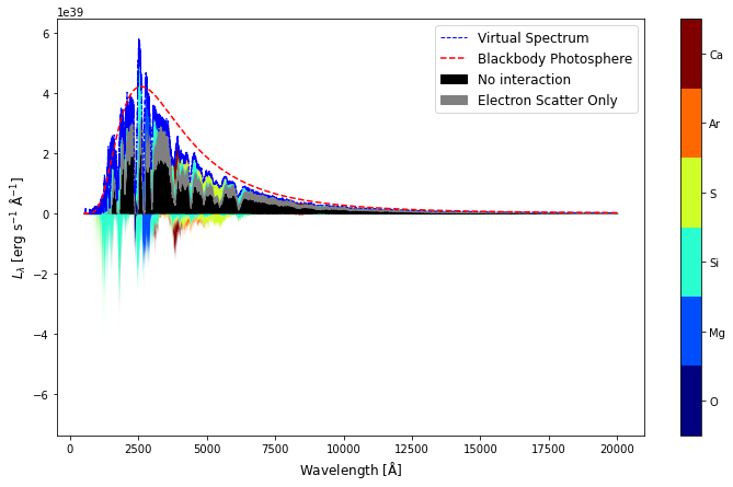
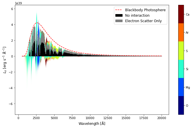
SDEC Plot illustrates the contributions of different chemical elements in the formation of a simulation model’s spectrum. It is a spectral diagnostic plot similar to those originally proposed by M. Kromer (see, for example, Kromer et al. 2013, figure 4).
First create a simulation model for which you want to generate this plot:
[2]:
from tardis import run_tardis
sim = run_tardis("tardis_example.yml")
[tardis.plasma.standard_plasmas][INFO ] Reading Atomic Data from kurucz_cd23_chianti_H_He.h5 (standard_plasmas.py:91)
[tardis.io.atom_data.util][INFO ] Atom Data kurucz_cd23_chianti_H_He.h5 not found in local path. Exists in TARDIS Data repo /home/atharva/Downloads/tardis-data/kurucz_cd23_chianti_H_He.h5 (util.py:34)
[tardis.io.atom_data.base][INFO ] Read Atom Data with UUID=6f7b09e887a311e7a06b246e96350010 and MD5=864f1753714343c41f99cb065710cace. (base.py:179)
[tardis.io.atom_data.base][INFO ] Non provided atomic data: synpp_refs, photoionization_data, yg_data, two_photon_data (base.py:183)
[tardis.simulation.base][INFO ] Starting iteration 1/20 (base.py:323)
Running post-merge numba montecarlo (with C close lines)!
[tardis.simulation.base][INFO ] Luminosity emitted = 7.94275e+42 erg / s Luminosity absorbed = 2.65805e+42 erg / s Luminosity requested = 1.05928e+43 erg / s (base.py:438)
[tardis.simulation.base][INFO ] Plasma stratification:
t_rad next_t_rad w next_w
Shell
0 9926.501965 10134.733717 0.400392 0.508204
5 9852.611678 10222.890845 0.211205 0.197026
10 9779.813302 10144.463169 0.142695 0.117179
15 9708.082813 9873.477846 0.104556 0.086941
(base.py:433)
[tardis.simulation.base][INFO ] t_inner 9933.952 K -- next t_inner 11472.055 K (base.py:434)
[tardis.simulation.base][INFO ] Starting iteration 2/20 (base.py:323)
Running post-merge numba montecarlo (with C close lines)!
[tardis.simulation.base][INFO ] Luminosity emitted = 1.40815e+43 erg / s Luminosity absorbed = 4.77001e+42 erg / s Luminosity requested = 1.05928e+43 erg / s (base.py:438)
[tardis.simulation.base][INFO ] Plasma stratification:
t_rad next_t_rad w next_w
Shell
0 10134.733717 11468.021903 0.508204 0.548671
5 10222.890845 11499.835340 0.197026 0.221374
10 10144.463169 11306.370330 0.117179 0.136291
15 9873.477846 10953.828130 0.086941 0.102617
(base.py:433)
[tardis.simulation.base][INFO ] t_inner 11472.055 K -- next t_inner 9949.978 K (base.py:434)
[tardis.simulation.base][INFO ] Starting iteration 3/20 (base.py:323)
Running post-merge numba montecarlo (with C close lines)!
[tardis.simulation.base][INFO ] Luminosity emitted = 8.12624e+42 erg / s Luminosity absorbed = 2.54722e+42 erg / s Luminosity requested = 1.05928e+43 erg / s (base.py:438)
[tardis.simulation.base][INFO ] Plasma stratification:
t_rad next_t_rad w next_w
Shell
0 11468.021903 10497.008397 0.548671 0.442299
5 11499.835340 10799.075913 0.221374 0.164288
10 11306.370330 10623.433274 0.136291 0.101820
15 10953.828130 10226.187071 0.102617 0.077629
(base.py:433)
[tardis.simulation.base][INFO ] t_inner 9949.978 K -- next t_inner 11360.097 K (base.py:434)
[tardis.simulation.base][INFO ] Starting iteration 4/20 (base.py:323)
Running post-merge numba montecarlo (with C close lines)!
[tardis.simulation.base][INFO ] Luminosity emitted = 1.36297e+43 erg / s Luminosity absorbed = 4.49721e+42 erg / s Luminosity requested = 1.05928e+43 erg / s (base.py:438)
[tardis.simulation.base][INFO ] Plasma stratification:
t_rad next_t_rad w next_w
Shell
0 10497.008397 11615.344313 0.442299 0.497714
5 10799.075913 11729.411389 0.164288 0.199205
10 10623.433274 11517.190317 0.101820 0.123849
15 10226.187071 11103.373456 0.077629 0.093930
(base.py:433)
[tardis.simulation.base][INFO ] t_inner 11360.097 K -- next t_inner 10014.843 K (base.py:434)
[tardis.simulation.base][INFO ] Starting iteration 5/20 (base.py:323)
Running post-merge numba montecarlo (with C close lines)!
[tardis.simulation.base][INFO ] Luminosity emitted = 8.27895e+42 erg / s Luminosity absorbed = 2.66933e+42 erg / s Luminosity requested = 1.05928e+43 erg / s (base.py:438)
[tardis.simulation.base][INFO ] Plasma stratification:
t_rad next_t_rad w next_w
Shell
0 11615.344313 10549.514128 0.497714 0.443441
5 11729.411389 10919.073481 0.199205 0.162199
10 11517.190317 10697.303300 0.123849 0.101289
15 11103.373456 10379.863073 0.093930 0.075372
(base.py:433)
[tardis.simulation.base][INFO ] t_inner 10014.843 K -- next t_inner 11328.210 K (base.py:434)
[tardis.simulation.base][INFO ] Starting iteration 6/20 (base.py:323)
Running post-merge numba montecarlo (with C close lines)!
[tardis.simulation.base][INFO ] Luminosity emitted = 1.34741e+43 erg / s Luminosity absorbed = 4.44727e+42 erg / s Luminosity requested = 1.05928e+43 erg / s (base.py:438)
[tardis.simulation.base][INFO ] Plasma stratification:
t_rad next_t_rad w next_w
Shell
0 10549.514128 11567.208184 0.443441 0.504178
5 10919.073481 11653.124121 0.162199 0.203042
10 10697.303300 11425.955010 0.101289 0.125249
15 10379.863073 11082.155938 0.075372 0.094028
(base.py:433)
[tardis.simulation.base][INFO ] t_inner 11328.210 K -- next t_inner 10044.200 K (base.py:434)
[tardis.simulation.base][INFO ] Starting iteration 7/20 (base.py:323)
Running post-merge numba montecarlo (with C close lines)!
[tardis.simulation.base][INFO ] Luminosity emitted = 8.39001e+42 erg / s Luminosity absorbed = 2.69230e+42 erg / s Luminosity requested = 1.05928e+43 erg / s (base.py:438)
[tardis.simulation.base][INFO ] Plasma stratification:
t_rad next_t_rad w next_w
Shell
0 11567.208184 10569.747403 0.504178 0.442290
5 11653.124121 11099.194259 0.203042 0.153253
10 11425.955010 10809.397890 0.125249 0.097256
15 11082.155938 10454.841299 0.094028 0.073809
(base.py:433)
[tardis.simulation.base][INFO ] t_inner 10044.200 K -- next t_inner 11285.966 K (base.py:434)
[tardis.simulation.base][INFO ] Starting iteration 8/20 (base.py:323)
Running post-merge numba montecarlo (with C close lines)!
[tardis.simulation.base][INFO ] Luminosity emitted = 1.33305e+43 erg / s Luminosity absorbed = 4.33011e+42 erg / s Luminosity requested = 1.05928e+43 erg / s (base.py:438)
[tardis.simulation.base][INFO ] Plasma stratification:
t_rad next_t_rad w next_w
Shell
0 10569.747403 11547.678162 0.442290 0.500345
5 11099.194259 11669.739508 0.153253 0.198338
10 10809.397890 11493.569590 0.097256 0.121915
15 10454.841299 11083.769586 0.073809 0.092834
(base.py:433)
[tardis.simulation.base][INFO ] t_inner 11285.966 K -- next t_inner 10060.511 K (base.py:434)
[tardis.simulation.base][INFO ] Starting iteration 9/20 (base.py:323)
Running post-merge numba montecarlo (with C close lines)!
[tardis.simulation.base][INFO ] Luminosity emitted = 8.44283e+42 erg / s Luminosity absorbed = 2.70894e+42 erg / s Luminosity requested = 1.05928e+43 erg / s (base.py:438)
[tardis.simulation.base][INFO ] Plasma stratification:
t_rad next_t_rad w next_w
Shell
0 11547.678162 10635.099217 0.500345 0.439520
5 11669.739508 11035.731464 0.198338 0.158320
10 11493.569590 10717.471486 0.121915 0.101642
15 11083.769586 10404.049299 0.092834 0.075794
(base.py:433)
[tardis.simulation.base][INFO ] t_inner 10060.511 K -- next t_inner 11268.877 K (base.py:434)
[tardis.simulation.base][INFO ] Starting iteration 10/20 (base.py:323)
Running post-merge numba montecarlo (with C close lines)!
[tardis.simulation.base][INFO ] Luminosity emitted = 1.32925e+43 erg / s Luminosity absorbed = 4.25943e+42 erg / s Luminosity requested = 1.05928e+43 erg / s (base.py:438)
[tardis.simulation.base][INFO ] Plasma stratification:
t_rad next_t_rad w next_w
Shell
0 10635.099217 11500.557678 0.439520 0.506895
5 11035.731464 11715.267406 0.158320 0.196690
10 10717.471486 11451.270656 0.101642 0.123243
15 10404.049299 11094.423438 0.075794 0.092243
(base.py:433)
[tardis.simulation.base][INFO ] t_inner 11268.877 K -- next t_inner 10059.624 K (base.py:434)
[tardis.simulation.base][INFO ] Starting iteration 11/20 (base.py:323)
Running post-merge numba montecarlo (with C close lines)!
[tardis.simulation.base][INFO ] Luminosity emitted = 8.49497e+42 erg / s Luminosity absorbed = 2.65616e+42 erg / s Luminosity requested = 1.05928e+43 erg / s (base.py:438)
[tardis.simulation.base][INFO ] Plasma stratification:
t_rad next_t_rad w next_w
Shell
0 11500.557678 10570.856509 0.506895 0.445926
5 11715.267406 10957.336276 0.196690 0.162837
10 11451.270656 10916.410391 0.123243 0.096229
15 11094.423438 10441.053929 0.092243 0.075026
(base.py:433)
[tardis.simulation.base][INFO ] t_inner 10059.624 K -- next t_inner 11233.248 K (base.py:434)
[tardis.simulation.base][INFO ] Starting iteration 12/20 (base.py:323)
Running post-merge numba montecarlo (with C close lines)!
[tardis.simulation.base][INFO ] Luminosity emitted = 1.30417e+43 erg / s Luminosity absorbed = 4.28820e+42 erg / s Luminosity requested = 1.05928e+43 erg / s (base.py:438)
[tardis.simulation.base][INFO ] Plasma stratification:
t_rad next_t_rad w next_w
Shell
0 10570.856509 11533.554419 0.445926 0.494814
5 10957.336276 11764.967895 0.162837 0.189464
10 10916.410391 11444.191999 0.096229 0.121150
15 10441.053929 11084.736033 0.075026 0.090825
(base.py:433)
[tardis.simulation.base][INFO ] t_inner 11233.248 K -- next t_inner 10123.784 K (base.py:434)
[tardis.simulation.base][INFO ] Starting iteration 13/20 (base.py:323)
Running post-merge numba montecarlo (with C close lines)!
[tardis.simulation.base][INFO ] Luminosity emitted = 8.69244e+42 erg / s Luminosity absorbed = 2.74548e+42 erg / s Luminosity requested = 1.05928e+43 erg / s (base.py:438)
[tardis.simulation.base][INFO ] Plasma stratification:
t_rad next_t_rad w next_w
Shell
0 11533.554419 10680.784661 0.494814 0.439281
5 11764.967895 10887.379428 0.189464 0.170137
10 11444.191999 10825.792025 0.121150 0.100780
15 11084.736033 10402.120228 0.090825 0.077634
(base.py:433)
[tardis.simulation.base][INFO ] t_inner 10123.784 K -- next t_inner 11175.750 K (base.py:434)
[tardis.simulation.base][INFO ] Starting iteration 14/20 (base.py:323)
Running post-merge numba montecarlo (with C close lines)!
[tardis.simulation.base][INFO ] Luminosity emitted = 1.28354e+43 erg / s Luminosity absorbed = 4.15095e+42 erg / s Luminosity requested = 1.05928e+43 erg / s (base.py:438)
[tardis.simulation.base][INFO ] Plasma stratification:
t_rad next_t_rad w next_w
Shell
0 10680.784661 11437.188130 0.439281 0.496749
5 10887.379428 11571.106856 0.170137 0.196714
10 10825.792025 11378.137918 0.100780 0.120954
15 10402.120228 10957.211814 0.077634 0.092896
(base.py:433)
[tardis.simulation.base][INFO ] t_inner 11175.750 K -- next t_inner 10152.603 K (base.py:434)
[tardis.simulation.base][INFO ] Starting iteration 15/20 (base.py:323)
Running post-merge numba montecarlo (with C close lines)!
[tardis.simulation.base][INFO ] Luminosity emitted = 8.75331e+42 erg / s Luminosity absorbed = 2.81319e+42 erg / s Luminosity requested = 1.05928e+43 erg / s (base.py:438)
[tardis.simulation.base][INFO ] Plasma stratification:
t_rad next_t_rad w next_w
Shell
0 11437.188130 10637.774893 0.496749 0.452668
5 11571.106856 11002.647927 0.196714 0.166197
10 11378.137918 10832.042108 0.120954 0.101284
15 10957.211814 10350.602742 0.092896 0.079468
(base.py:433)
[tardis.simulation.base][INFO ] t_inner 10152.603 K -- next t_inner 11168.529 K (base.py:434)
[tardis.simulation.base][INFO ] Starting iteration 16/20 (base.py:323)
Running post-merge numba montecarlo (with C close lines)!
[tardis.simulation.base][INFO ] Luminosity emitted = 1.27820e+43 erg / s Luminosity absorbed = 4.15606e+42 erg / s Luminosity requested = 1.05928e+43 erg / s (base.py:438)
[tardis.simulation.base][INFO ] Plasma stratification:
t_rad next_t_rad w next_w
Shell
0 10637.774893 11420.979987 0.452668 0.499488
5 11002.647927 11711.923994 0.166197 0.186857
10 10832.042108 11421.346118 0.101284 0.119700
15 10350.602742 11076.434180 0.079468 0.089402
(base.py:433)
[tardis.simulation.base][INFO ] t_inner 11168.529 K -- next t_inner 10167.208 K (base.py:434)
[tardis.simulation.base][INFO ] Starting iteration 17/20 (base.py:323)
Running post-merge numba montecarlo (with C close lines)!
[tardis.simulation.base][INFO ] Luminosity emitted = 8.81647e+42 erg / s Luminosity absorbed = 2.81681e+42 erg / s Luminosity requested = 1.05928e+43 erg / s (base.py:438)
[tardis.simulation.base][INFO ] Plasma stratification:
t_rad next_t_rad w next_w
Shell
0 11420.979987 10691.849845 0.499488 0.447482
5 11711.923994 11042.045712 0.186857 0.164090
10 11421.346118 10980.886609 0.119700 0.097369
15 11076.434180 10456.662007 0.089402 0.077097
(base.py:433)
[tardis.simulation.base][INFO ] t_inner 10167.208 K -- next t_inner 11144.459 K (base.py:434)
[tardis.simulation.base][INFO ] Starting iteration 18/20 (base.py:323)
Running post-merge numba montecarlo (with C close lines)!
[tardis.simulation.base][INFO ] Luminosity emitted = 1.26680e+43 erg / s Luminosity absorbed = 4.12238e+42 erg / s Luminosity requested = 1.05928e+43 erg / s (base.py:438)
[tardis.simulation.base][INFO ] Plasma stratification:
t_rad next_t_rad w next_w
Shell
0 10691.849845 11404.686443 0.447482 0.497739
5 11042.045712 11664.227712 0.164090 0.189070
10 10980.886609 11444.220669 0.097369 0.117732
15 10456.662007 11052.698087 0.077097 0.089141
(base.py:433)
[tardis.simulation.base][INFO ] t_inner 11144.459 K -- next t_inner 10190.841 K (base.py:434)
[tardis.simulation.base][INFO ] Starting iteration 19/20 (base.py:323)
Running post-merge numba montecarlo (with C close lines)!
[tardis.simulation.base][INFO ] Luminosity emitted = 8.87081e+42 erg / s Luminosity absorbed = 2.87116e+42 erg / s Luminosity requested = 1.05928e+43 erg / s (base.py:438)
[tardis.simulation.base][INFO ] Plasma stratification:
t_rad next_t_rad w next_w
Shell
0 11404.686443 10732.832306 0.497739 0.444436
5 11664.227712 11084.302807 0.189070 0.162591
10 11444.220669 10899.736539 0.117732 0.099122
15 11052.698087 10465.941519 0.089141 0.077378
(base.py:433)
[tardis.simulation.base][INFO ] t_inner 10190.841 K -- next t_inner 11136.097 K (base.py:434)
[tardis.simulation.base][INFO ] Starting iteration 20/20 (base.py:323)
Running post-merge numba montecarlo (with C close lines)!
[tardis.simulation.base][INFO ] Luminosity emitted = 1.26319e+43 erg / s Luminosity absorbed = 4.10706e+42 erg / s Luminosity requested = 1.05928e+43 erg / s (base.py:438)
[tardis.simulation.base][INFO ] Simulation finished in 20 iterations and took 32.49 s (base.py:381)
Important: The virtual packet logging capability must be active in order to produce SDEC Plot for virtual packets population. Thus, make sure to set virtual_packet_logging: True in your configuration file if you want to generate SDEC Plot with virtual packets. It should be added under virtual property of spectrum property, as described in configuration schema.
Now, import the plotting interface for SDEC plot, i.e. SDECPlotter class.
[3]:
from tardis.visualization import SDECPlotter
And create a plotter object to process the data of simulation object sim for generating SDEC plots.
[4]:
plotter = SDECPlotter.from_simulation(sim)
Static Plot (in matplotlib)
You can now call generate_plot_mpl() method on your plotter object to get a highly informative, yet beautiful, SDEC plot produced in matplotlib.
Virtual packets mode
By default, SDEC plot is produced for the virtual packet population of the simulation.
[5]:
plotter.generate_plot_mpl();
Real packets mode
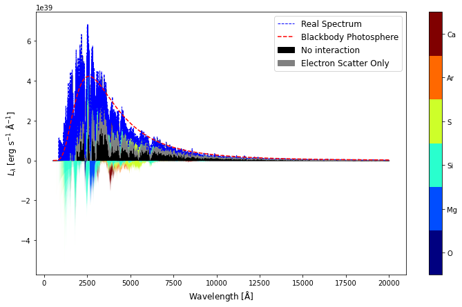
You can produce SDEC plot for the real packet population of the simulation by setting packets_mode="real" which is "virtual" by default. Since packets_mode is 1st argument, you can simply pass "real" string only.
[6]:
plotter.generate_plot_mpl("real");
Plotting a specific wavelength range
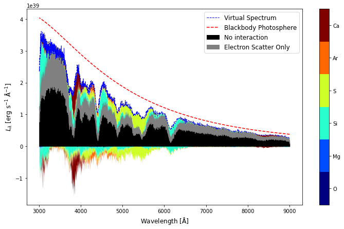
You can also restrict the wavelength range of escaped packets that you want to plot by specifying packet_wvl_range. It should be a quantity having units of Angstrom, containing two values - lower lambda and upper lambda i.e. [lower_lambda, upper_lambda] * u.AA.
[7]:
from astropy import units as u
[8]:
plotter.generate_plot_mpl(packet_wvl_range=[3000, 9000] * u.AA);
Plotting flux instead of luminosity
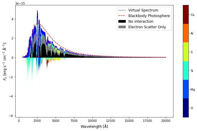
You can plot in units of flux on the Y-axis of the SDEC plot, by specifying the distance parameter. It should be a quantity with a unit of length like m, Mpc, etc. and must be a positive value. By default, distance=None plots luminosity on the Y-axis.
[9]:
plotter.generate_plot_mpl(distance=100 * u.Mpc);
Hiding modeled spectrum
By default, modeled spectrum is shown in SDEC plot. You can hide it by setting show_modeled_spectrum=False.
[10]:
plotter.generate_plot_mpl(show_modeled_spectrum=False);
Additional plotting options
[11]:
# To list all avaialble options (or parameters) with their description
help(plotter.generate_plot_mpl)
Help on method generate_plot_mpl in module tardis.visualization.tools.sdec_plot:
generate_plot_mpl(packets_mode='virtual', packet_wvl_range=None, distance=None, show_modeled_spectrum=True, ax=None, figsize=(12, 7), cmapname='jet', nelements=None, species_list=None) method of tardis.visualization.tools.sdec_plot.SDECPlotter instance
Generate Spectral element DEComposition (SDEC) Plot using matplotlib.
Parameters
----------
packets_mode : {'virtual', 'real'}, optional
Mode of packets to be considered, either real or virtual. Default
value is 'virtual'
packet_wvl_range : astropy.Quantity or None, optional
Wavelength range to restrict the analysis of escaped packets. It
should be a quantity having units of Angstrom, containing two
values - lower lambda and upper lambda i.e.
[lower_lambda, upper_lambda] * u.AA. Default value is None
distance : astropy.Quantity or None, optional
Distance used to calculate flux instead of luminosity in the plot.
It should have a length unit like m, Mpc, etc. Default value is None
show_modeled_spectrum : bool, optional
Whether to show modeled spectrum in SDEC Plot. Default value is
True
ax : matplotlib.axes._subplots.AxesSubplot or None, optional
Axis on which to create plot. Default value is None which will
create plot on a new figure's axis.
figsize : tuple, optional
Size of the matplotlib figure to display. Default value is (12, 7)
cmapname : str, optional
Name of matplotlib colormap to be used for showing elements.
Default value is "jet"
nelements: int
Number of elements to include in plot. Determined by the
largest contribution to total luminosity absorbed and emitted.
Other elements are shown in silver. Default value is
None, which displays all elements
species_list: list of strings or None
list of strings containing the names of species that should be included in the SDEC plots.
Must be given in Roman numeral format. Can include specific ions, a range of ions,
individual elements, or any combination of these:
e.g. ['Si II', 'Ca II', 'C', 'Fe I-V']
Returns
-------
matplotlib.axes._subplots.AxesSubplot
Axis on which SDEC Plot is created
The generate_plot_mpl method also has options specific to the matplotlib API, thereby providing you more control over how your SDEC plot looks. Possible cases where you may use them are:
ax: To plot SDEC on the Axis of a plot you’re already working with, e.g. for subplots.figsize: To resize SDEC plot as per your requirements.cmapname: To use a colormap of your preference, instead of “jet”.
Interactive Plot (in plotly)
If you’re using SDEC plot for exploration purposes, you should plot its interactive version by using generate_plot_ply(). This not only allows you to zoom & pan but also to inspect data values by hovering, to resize scale, etc. conveniently (as shown below).
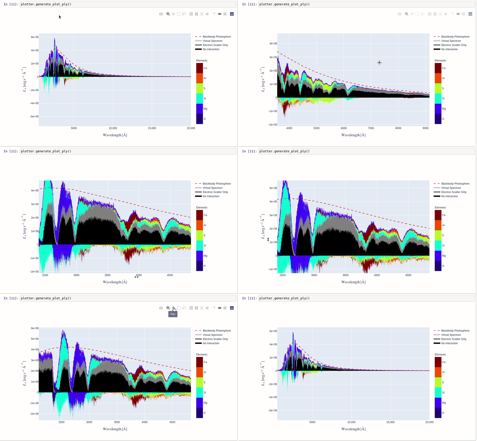
This method takes exact same arguments as generate_plot_mpl except a few that are specific to the plotting library. We can produce all the plots above in plotly, by passing the same arguments.
Plotting a specific wavelength range
[14]:
plotter.generate_plot_ply(packet_wvl_range=[3000, 9000] * u.AA)
In similar manner, you can also use show_modeled_spectrum and distance argument in plotly plots.
Additional plotting options
[15]:
# To list all avaialble options (or parameters) with their description
help(plotter.generate_plot_ply)
Help on method generate_plot_ply in module tardis.visualization.tools.sdec_plot:
generate_plot_ply(packets_mode='virtual', packet_wvl_range=None, distance=None, observed_spectrum=None, show_modeled_spectrum=True, fig=None, graph_height=600, cmapname='jet', nelements=None, species_list=None) method of tardis.visualization.tools.sdec_plot.SDECPlotter instance
Generate interactive Spectral element DEComposition (SDEC) Plot using plotly.
Parameters
----------
packets_mode : {'virtual', 'real'}, optional
Mode of packets to be considered, either real or virtual. Default
value is 'virtual'
packet_wvl_range : astropy.Quantity or None, optional
Wavelength range to restrict the analysis of escaped packets. It
should be a quantity having units of Angstrom, containing two
values - lower lambda and upper lambda i.e.
[lower_lambda, upper_lambda] * u.AA. Default value is None
distance : astropy.Quantity or None, optional
Distance used to calculate flux instead of luminosity in the plot.
It should have a length unit like m, Mpc, etc. Default value is None
show_modeled_spectrum : bool, optional
Whether to show modeled spectrum in SDEC Plot. Default value is
True
fig : plotly.graph_objs._figure.Figure or None, optional
Figure object on which to create plot. Default value is None which
will create plot on a new Figure object.
graph_height : int, optional
Height (in px) of the plotly graph to display. Default value is 600
cmapname : str, optional
Name of the colormap to be used for showing elements.
Default value is "jet"
nelements: int
Number of elements to include in plot. Determined by the
largest contribution to total luminosity absorbed and emitted.
Other elements are shown in silver. Default value is
None, which displays all elements
species_list: list of strings or None
list of strings containing the names of species that should be included in the SDEC plots.
Must be given in Roman numeral format. Can include specific ions, a range of ions,
individual elements, or any combination of these:
e.g. ['Si II', 'Ca II', 'C', 'Fe I-V']
Returns
-------
plotly.graph_objs._figure.Figure
Figure object on which SDEC Plot is created
The generate_plot_ply method also has options specific to the plotly API, thereby providing you more control over how your SDEC plot looks. Possible cases where you may use them are: - fig: To plot SDEC on a figure you are already using e.g. for subplots. - graph_height: To specify the height of graph as needed. - cmapname: To use colormap of your preference instead of “jet”.
Using simulation saved as HDF
Other than producing SDEC Plot for simulation objects in runtime, you can also produce it for saved TARDIS simulations.
[16]:
hdf_plotter = SDECPlotter.from_hdf("demo.hdf")
This hdf_plotter object is similar to the plotter object we used above, so you can use each plotting method demonstrated above with this too.
[17]:
# Static plot with virtual packets mode
hdf_plotter.generate_plot_mpl();

[18]:
# Static plot with real packets mode
hdf_plotter.generate_plot_mpl("real");

[19]:
# Interactive plot with virtual packets mode
hdf_plotter.generate_plot_ply()
[ ]: